Inspect local sharpness
Compute a Laplacian response, square it and average locally to visualize high-frequency energy.
The pipeline
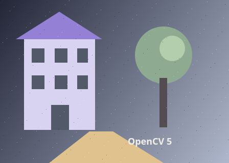
The unchanged source image. All steps use this same example.
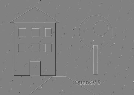
Second derivatives emphasize high-frequency structure.
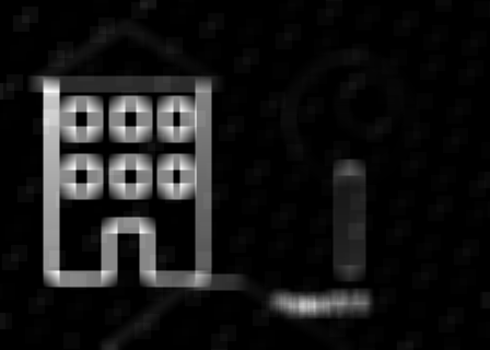
Mean squared Laplacian response in each window, normalized here for display. The final preview uses this same image; numeric energy remains available in the lab inspector.
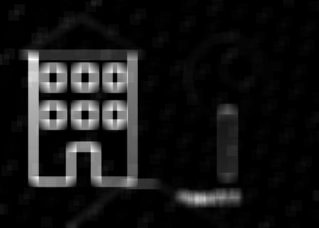
Mean local energy 5676.557 intensity². Texture and noise also increase this value.
Measure second derivatives
Explore the algorithm →LaplacianA signed Laplacian highlights rapid intensity changes.
- Receives
- Grayscale intensity.
- Passes to the next step
- A signed derivative field.
Why this step? The Laplacian is a second spatial derivative and responds strongly around rapid transitions. A float32 destination retains both signs instead of clipping one side of an edge.
Measure local energy
Explore the algorithm →multiplyblurSquare responses and average in a neighbourhood.
- Receives
- The signed derivative values.
- Passes to the next step
- A float32 mean-squared-Laplacian map in intensity-squared units.
Why this step? Squaring turns both positive and negative responses into nonnegative energy. Box averaging summarizes energy in a local neighbourhood, so a window receives a score rather than alternating signs that would cancel.
Visualize the field
Explore the algorithm →normalizeNormalize the energy for display; retain numeric values for inspection.
- Receives
- The local energy map.
- Produces
- A visible sharpness-related map and its original local energy values.
Why this step? Min-max normalization maps the field into an 8-bit preview so its spatial pattern is visible. The lab keeps native values for numeric inspection. This is display scaling, not histogram equalization, and it does not calibrate the score across images.
Actual OpenCV 5.0.0 results on the illustrated sample, using the lab’s default algorithm settings. Masks, overlays and normalized fields are labelled previews; the data contracts above describe what the algorithms really exchange. Try this chain with your images ↓
Why this chain works
Blur weakens rapid intensity changes. A derivative-energy map can show where those changes remain, but the result is also driven by how much texture and noise the scene contains.
- 01
Measure second derivatives
LaplacianThe Laplacian is a second spatial derivative and responds strongly around rapid transitions. A float32 destination retains both signs instead of clipping one side of an edge.
- Receives
- Grayscale intensity.
- Passes on
- A signed derivative field.
- 02
Measure local energy
multiplyblurSquaring turns both positive and negative responses into nonnegative energy. Box averaging summarizes energy in a local neighbourhood, so a window receives a score rather than alternating signs that would cancel.
- Receives
- The signed derivative values.
- Passes on
- A float32 mean-squared-Laplacian map in intensity-squared units.
- 03
Visualize the field
normalizeMin-max normalization maps the field into an 8-bit preview so its spatial pattern is visible. The lab keeps native values for numeric inspection. This is display scaling, not histogram equalization, and it does not calibrate the score across images.
- Receives
- The local energy map.
- Passes on
- A visible sharpness-related map and its original local energy values.
Tune and diagnose
Choose the parameters
A small energy window gives a localized but noisier map; a large window smooths the score across features. Keep image size, exposure and processing settings fixed when comparing numeric values across a sequence.
Read the result
A blank but sharply focused wall can score below a blurry patterned surface. Noise also raises the score. Compare the same textured region across candidate frames rather than treating the map as universal image quality.
Try it with your images
Choose your own image or start with the built-in sample. Run the recipe, then use the stage buttons to inspect intermediate results without rerunning it.
Experiment at pixel level
Compute a Laplacian response, square it and average locally to visualize high-frequency energy.
The engine loads on your first run. Your images stay in this browser.
Scroll over either image to zoom at the pointer. Use the scrollbars to pan both views over the same relative area. Zoom is relative to the input; pixel coordinates belong to each image. Warps can change scene correspondence.
Pixel inspector RGBA · native values · matched scale · 9 × 9 output pixels
Select a pixel
Select a pixel
Assumptions and limits
Texture and noise increase this score too. It is not a calibrated focus or perceptual quality measurement.
TypeScript core chain
Initialize the shared engine once with await initOpenCV(), then use these named imports. In a bundled browser app, pass the WASM URL as shown in the quickstart. image is an 8-bit BGR Mat from that same engine; paired recipes receive an equally sized nextImage. Region recipes use an in-bounds pixel rect. Read outputs before the using scope ends. See matrix ownership.
import {
  COLOR_BGR2GRAY,
  CV_32F,
  CV_8U,
  Laplacian,
  Mat,
  NORM_MINMAX,
  blur,
  cvtColor,
  mean,
  multiply,
  normalize
} from '@banou/opencv-wasm'

// The engine is already initialized; image is an 8-bit BGR Mat.
// "using" releases native handles at scope exit; inspect or copy outputs before then.

// Allocate brightness, a signed derivative, numeric energy and a display-only image.
using gray = new Mat(), derivative = new Mat(), energy = new Mat(), display = new Mat()
// Measure changes in brightness without mixing separate colour-channel scores.
cvtColor(image, gray, COLOR_BGR2GRAY)
// 1. A 3x3 Laplacian emphasizes rapid spatial changes. CV_32F preserves
// negative as well as positive responses; unsigned output would clip negatives.
Laplacian(gray, derivative, CV_32F, 3)
// 2. Square the derivative pointwise so opposite signs add energy instead of cancelling.
multiply(derivative, derivative, energy)
// Average that energy in a 15x15 window to obtain a local, less noisy score.
blur(energy, energy, { width: 15, height: 15 })
// 3. Map this image's minimum/maximum energy to 0..255 only for visualization.
// Keep the float energy Mat for real measurements; display brightness is not an absolute score.
normalize(energy, display, 0, 255, NORM_MINMAX, CV_8U)
// Report the mean native energy. Texture and noise also raise it, so compare
// the same scene region at the same resolution when using it to assess focus.
console.log('Mean squared Laplacian:', mean(energy)[0])
The snippets isolate the core operations. The complete runnable recipes also include validation, filtering, overlays, intermediate previews and resource cleanup.