Simplify an image into colour regions
Smooth small colour fluctuations, cluster colours with k-means and render the reduced palette.
The pipeline
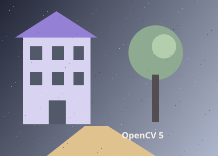
The unchanged source image. All steps use this same example.
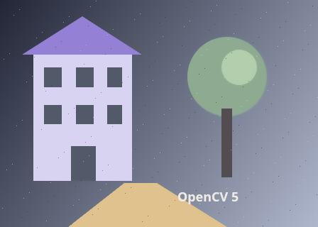
Bilateral filtering reduces within-region variation before clustering.

Each swatch is one learned BGR cluster centre. Cluster IDs assign every image pixel to one of these colours.
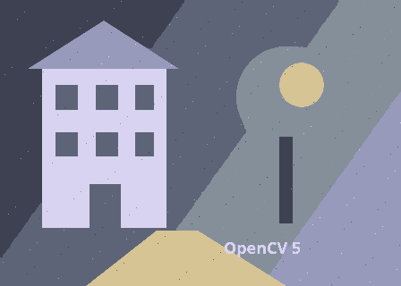
Reduced to 6 learned BGR colours.
Smooth within colour regions
Explore the algorithm →bilateralFilterBilateral filtering reduces small variations while retaining boundaries.
- Receives
- An 8-bit BGR image.
- Passes to the next step
- A smoothed colour image.
Why this step? Bilateral filtering averages nearby pixels according to both position and colour similarity. This reduces fluctuations within colour regions while preserving some strong boundaries, giving clustering fewer small variations to spend palette entries on.
Learn a palette
Explore the algorithm →kmeansKMEANS_PP_CENTERSK-means groups BGR colour samples into clusters.
- Receives
- A float32 sample matrix with one BGR triplet per pixel.
- Passes to the next step
- One integer cluster ID per pixel and K learned BGR centres.
Why this step? K-means alternates assigning pixels to their nearest colour centre and updating centres from assigned samples. K-means++ chooses spread-out initial centres. The lab clusters colour only, so disconnected areas of similar colour can share the same palette entry.
Recolour the image
Explore the algorithm →Palette lookupReplace each pixel with its assigned cluster centre.
- Receives
- Cluster labels and colour centres.
- Produces
- A quantized colour image and inspectable palette IDs.
Why this step? Replacing each pixel by its assigned centre turns the learned clusters into a visible reduced-palette image. Keeping the label field allows later grouping, recolouring or measuring palette usage without reclustering.
Actual OpenCV 5.0.0 results on the illustrated sample, using the lab’s default algorithm settings. Masks, overlays and normalized fields are labelled previews; the data contracts above describe what the algorithms really exchange. Try this chain with your images ↓
Why this chain works
To summarize an image with a small set of colours, first reduce incidental local variation, then learn representative colours and assign every pixel to one of them.
- 01
Smooth within colour regions
bilateralFilterBilateral filtering averages nearby pixels according to both position and colour similarity. This reduces fluctuations within colour regions while preserving some strong boundaries, giving clustering fewer small variations to spend palette entries on.
- Receives
- An 8-bit BGR image.
- Passes on
- A smoothed colour image.
- 02
Learn a palette
kmeansKMEANS_PP_CENTERSK-means alternates assigning pixels to their nearest colour centre and updating centres from assigned samples. K-means++ chooses spread-out initial centres. The lab clusters colour only, so disconnected areas of similar colour can share the same palette entry.
- Receives
- A float32 sample matrix with one BGR triplet per pixel.
- Passes on
- One integer cluster ID per pixel and K learned BGR centres.
- 03
Recolour the image
Palette lookupReplacing each pixel by its assigned centre turns the learned clusters into a visible reduced-palette image. Keeping the label field allows later grouping, recolouring or measuring palette usage without reclustering.
- Receives
- Cluster labels and colour centres.
- Passes on
- A quantized colour image and inspectable palette IDs.
Tune and diagnose
Choose the parameters
Increase palette colours to retain more distinctions; decrease them for stronger simplification. Increase bilateral colour sigma to smooth a broader range of colours before clustering, while watching for merging of important boundaries.
Read the result
K-means optimizes sample distances, not semantic importance or perceptual colour difference. A small but important accent colour may disappear. For perceptual palette work, consider clustering in Lab and handling conversion and gamut deliberately.
Try it with your images
Choose your own image or start with the built-in sample. Run the recipe, then use the stage buttons to inspect intermediate results without rerunning it.
Experiment at pixel level
Smooth small colour fluctuations, cluster colours with k-means and render the reduced palette.
The engine loads on your first run. Your images stay in this browser.
Scroll over either image to zoom at the pointer. Use the scrollbars to pan both views over the same relative area. Zoom is relative to the input; pixel coordinates belong to each image. Warps can change scene correspondence.
Pixel inspector RGBA · native values · matched scale · 9 × 9 output pixels
Select a pixel
Select a pixel
Assumptions and limits
Results depend on the image’s colour distribution. Small but significant colours may disappear into larger clusters.
TypeScript core chain
Initialize the shared engine once with await initOpenCV(), then use these named imports. In a bundled browser app, pass the WASM URL as shown in the quickstart. image is an 8-bit BGR Mat from that same engine; paired recipes receive an equally sized nextImage. Region recipes use an in-bounds pixel rect. Read outputs before the using scope ends. See matrix ownership.
import {
  CV_32F,
  KMEANS_PP_CENTERS,
  Mat,
  TERM_CRITERIA_COUNT,
  TERM_CRITERIA_EPS,
  bilateralFilter,
  kmeans
} from '@banou/opencv-wasm'

// The engine is already initialized; image is an 8-bit BGR Mat.
// "using" releases native handles at scope exit; inspect or copy outputs before then.

// 1. Allocate an image with reduced variation inside colour regions.
using smooth = new Mat()
// Use a 7-pixel neighbourhood, colour sigma 40 and spatial sigma 5 pixels.
// Bilateral weights favour nearby, similar colours to smooth while retaining strong edges.
bilateralFilter(image, smooth, 7, 40, 5)
// 2. Each pixel becomes one sample row with three BGR values. CV_32F
// stores each component as a float, the format expected by k-means.
using samples = new Mat(smooth.rows * smooth.cols, 3, CV_32F)
// Copy interleaved 8-bit BGR components into float storage without changing their order.
samples.data32F.set(smooth.data)
// Allocate each sample's integer cluster ID and the learned BGR colour centres.
using labels = new Mat(), centres = new Mat()
// 3. Learn six colour groups. Stop after at most 20 updates or centre motion
// within epsilon 0.5; the flags enable both criteria. Use one attempt and
// k-means++ initialization to spread the starting centres across the samples.
kmeans(samples, 6, labels,
  { type: TERM_CRITERIA_COUNT | TERM_CRITERIA_EPS, maxCount: 20, epsilon: 0.5 },
  1, KMEANS_PP_CENTERS, centres)
// labels.data32S chooses a BGR triplet from centres.data32F for each pixel.
The snippets isolate the core operations. The complete runnable recipes also include validation, filtering, overlays, intermediate previews and resource cleanup.